–>	f(t) := if t>=0 and t < %pi/4 then 2·%pi else if t>=%pi/4 and t < %pi/2 then %pi else if t>=%pi/2 and t <= %pi then 0 else if t<0 and t>=−%pi then f(−t) else if t>0 then f(t − ceiling(t/(2·%pi))·2·%pi) else if t<0 then f(−t);

\[\tag{%o35} \operatorname{f}(t):=\operatorname{if} t\mbox{> =}0\mathit{ and }t\mbox{< }\frac{\ensuremath{\pi} }{4} \operatorname{then} 2 \ensuremath{\pi} \operatorname{else} \operatorname{if} t\mbox{> =}\frac{\ensuremath{\pi} }{4}\mathit{ and }t\mbox{< }\frac{\ensuremath{\pi} }{2} \operatorname{then} \ensuremath{\pi} \operatorname{else} \operatorname{if} t\mbox{> =}\frac{\ensuremath{\pi} }{2}\mathit{ and }t\mbox{< =}\ensuremath{\pi} \operatorname{then} 0 \operatorname{else} \operatorname{if} t\mbox{< }0\mathit{ and }t\mbox{> =}-\ensuremath{\pi} \operatorname{then} \operatorname{f}\left( -t\right) \operatorname{else} \operatorname{if} t\mbox{> }0 \operatorname{then} \operatorname{f}\left( t-\operatorname{ceiling}\left( \frac{t}{2 \ensuremath{\pi} }\right) 2 \ensuremath{\pi} \right) \operatorname{else} \operatorname{if} t\mbox{< }0 \operatorname{then} \operatorname{f}\left( -t\right) \]

–>

f(−4.9);

\[\tag{%o2} \ensuremath{\pi} \]

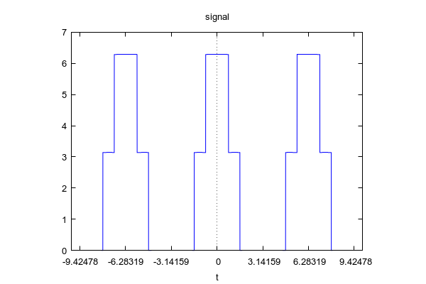
Courbe ( 3 périodes )

–>	wxplot2d( f(t), [t, −10, 10], [xtics, %pi], [title, "signal"]);

\[\tag{%t36} \]

\[\tag{%o36} \]

–>	load("draw");

\[\mbox{}\\\mbox{0 errors, 0 warnings}\]
\[\tag{%o38} /usr/local/share/maxima/5.41.0/share/draw/draw.lisp\]

Définition d’une fonction fsignal, paramétrée par n = nombre de termes de la série de fourier à prendre en considération

–>	fsignal(n, x)  := block([i], res : 3·%pi/4, for i from 1 thru n do (      res : res + (2/i) · ( sin(i·%pi/4) + sin(i·%pi/2)) · cos(i·x) ), res);

\[\tag{%o39} \operatorname{fsignal}\left( n,x\right) :=\operatorname{block}\left( [i],\mathit{res}:\frac{3 \ensuremath{\pi} }{4},\operatorname{for} i \operatorname{thru} n \operatorname{do} \mathit{res}:\mathit{res}+\frac{2}{i}\, \left( \sin{\left( \frac{i \ensuremath{\pi} }{4}\right) }+\sin{\left( \frac{i \ensuremath{\pi} }{2}\right) }\right) \cos{\left( i x\right) },\mathit{res}\right) \]

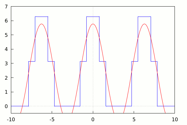
–>	fsignal(1,x);

\[\tag{%o40} 2 \left( \frac{1}{\sqrt{2}}+1\right) \cos{(x)}+\frac{3 \ensuremath{\pi} }{4}\]

–>	set_draw_defaults(   xaxis = true, xaxis_color = red,   xaxis_type = solid, xaxis_width = 1,  xtics=1,   yaxis = true, yaxis_color = red, ytics=1,   yaxis_type = solid, yaxis_width = 1,   dimensions = [600,600],   grid = true,   nticks = 150,   ip_grid = [100,100],   line_width = 3 );

\[\tag{%o41} [\mathit{xaxis}=\mbox{true},\mathit{xaxis\_ color}=\mathit{red},\mathit{xaxis\_ type}=\mathit{solid},\mathit{xaxis\_ width}=1,\mathit{xtics}=1,\mathit{yaxis}=\mbox{true},\mathit{yaxis\_ color}=\mathit{red},\mathit{ytics}=1,\mathit{yaxis\_ type}=\mathit{solid},\mathit{yaxis\_ width}=1,\mathit{dimensions}=[600,600],\mathit{grid}=\mbox{true},\mathit{nticks}=150,\mathit{ip\_ grid}=[100,100],\mathit{line\_ width}=3]\]

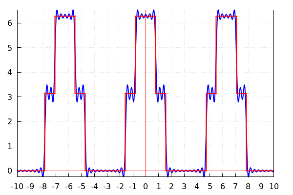
Traçage de la fonction ‘signal’ et de la somme Fourier au rang  n = 20

–>	wxdraw2d(color=blue,line_width=2,     explicit(fsignal(20,x),x,−10,10),     color=red,     explicit(f(x), x, −10, 10)    );

\[\tag{%t42} \]

\[\tag{%o42} \]

–>	with_slider_draw(k, makelist(i, i, 1, 15),    xrange=[−10, 10], yrange=[−0.5, 7],    xaxis = true, yaxis = true,    color = blue, explicit(f(x), x, −10, 10),    color = red, explicit(fsignal(k,x),x,−10,10) );

\[\tag{%t11} \]

\[\tag{%o11} \]

–>	makelist(1/n·cos(n·%pi/4) +1/n·cos(n·%pi/2), n, 1, 6);

\[\tag{%o13} [\frac{1}{\sqrt{2}},-\frac{1}{2},-\frac{1}{3 \sqrt{2}},0,-\frac{1}{5 \sqrt{2}},-\frac{1}{6}]\]