Maxima: champs tournants

Théorème de Ferraris – champs tournants

Le théorème de Ferraris démontre qu’un champ tournant peut être créé par trois bobines positionnées en arc de cercle avec un décalage de 120°, chacune alimentées par une phase d’un courant électrique triphasé1. La fréquence de rotation est alors égale à la fréquence de courants d’alimentation. Il démontre également que 3p bobines alimentées en triphasé et décalées de 120°/p permettent d’obtenir un champ tournant avec une fréquence de rotation f/p, f étant la fréquence des courants d’alimentation.

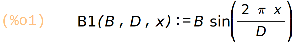
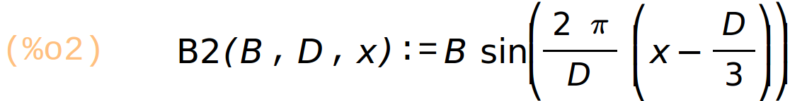
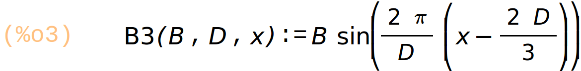
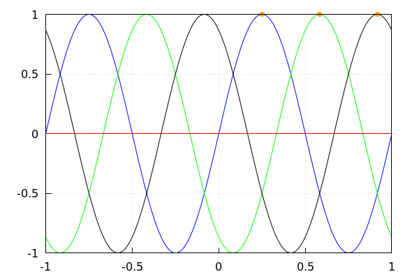
Définition de trois champs périodiques dans l’espace, période = D
champs B1, B2, B3 décalés de D/3


(%i3)

B1(B, D, x) := B·sin(2·%pi·x/D) ;
B2(B, D, x) := B·sin(2·%pi/D·(x D/3));
B3(B, D, x) := B·sin(2·%pi/D·(x 2·D/3));

(%o1) B1(B,D,x):=B*sin((2*%pi*x)/D)

(%o2) B2(B,D,x):=B*sin((2*%pi)/D*(x-D/3))

(%o3) B3(B,D,x):=B*sin((2*%pi)/D*(x-(2*D)/3))


(%i4)

sommeB(B, D, x) := B1(B,D,x) + B2(B,D,x) + B3(B,D,x);

(%o4) sommeB(B,D,x):=B1(B,D,x)+B2(B,D,x)+B3(B,D,x)


(%i6)

f : 50; T: 1/f;

(f) 50

(T) 1/50


(%i10)

load(draw);
D : 1;
line : [[D/4, 1], [D/3+D/4, 1], [2·D/3 + D/4, 1]];
wxdraw2d(
grid = true,
color=blue,  explicit(B1(1, 1,x), x, 1, 1),
color=green, explicit(B2(1,1,x),x, 1, 1),
color=black, explicit(B3(1,1,x),x, 1, 1),
color=red,   explicit(sommeB(1,1,x),x, 1, 1),
color=orange, point_type=7, points(line)
);

0 errors, 0 warnings

(%o7) "/usr/local/share/maxima/5.41.0/share/draw/draw.lisp"

(D) 1

(line) [[1/4,1],[7/12,1],[11/12,1]]

(%t10)

 (Graphics)

(%o10)


(%i11)

omega : 2·%pi·f;

(omega) 100*%pi


(%i12)

A0 : 1;

(A0) 1


(%i15)

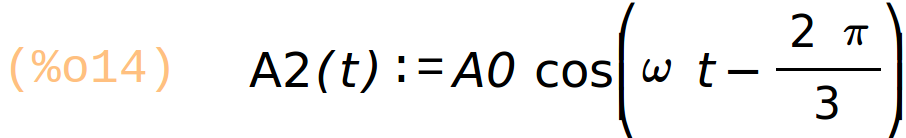
A1(t) := A0·cos(omega·t); A2(t) := A0·cos(omega·t 2·%pi/3); A3(t) := A0·cos(omega·t 4·%pi/3);

(%o13) A1(t):=A0*cos(omega*t)

(%o14) A2(t):=A0*cos(omega*t-(2*%pi)/3)

(%o15) A3(t):=A0*cos(omega*t-(4*%pi)/3)


(%i18)

champ1(x, t) := B1( A1(t), 1, x); champ2(x, t) := B2( A2(t), 1, x); champ3(x, t) := B3( A3(t), 1, x);

(%o16) champ1(x,t):=B1(A1(t),1,x)

(%o17) champ2(x,t):=B2(A2(t),1,x)

(%o18) champ3(x,t):=B3(A3(t),1,x)

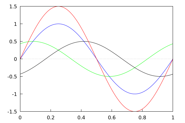
Traçage des 3 champs séparés, et de leur somme (en rouge).


(%i19)

with_slider_draw(k, makelist(i·T/32, i, 0, 32),
xrange=[0, 1], yrange=[1.5, 1.5],
xaxis = true, yaxis = true,
color = blue, explicit(champ1(x, k),x,0,1),
color = green, explicit(champ2(x, k),x,0,1),
color = black, explicit(champ3(x, k),x,0,1),
color=red,  explicit(  champ1(x, k)+champ2(x, k)+champ3(x, k)    , x,  0,  1)
);

(%t19)

Animated Diagram
(%o19)

À faire :

  1. Voyez ce qui ce passe lorsqu’on inverse deux champs
    par exemple, champ1(x, t) := B1( A2(t), 1, x);
    et champ2(x, t) := B2( A1(t), 1, x);
  2. Proposez un moteur à 2 phases.

Polynômes de Lagrange – wxMaxima


Fonction périodique – Fourier (SNIR2)


Signal défini par une fonction paire 2 PI périodique

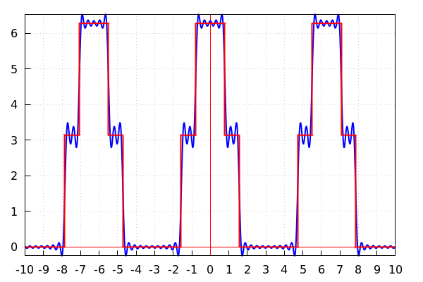
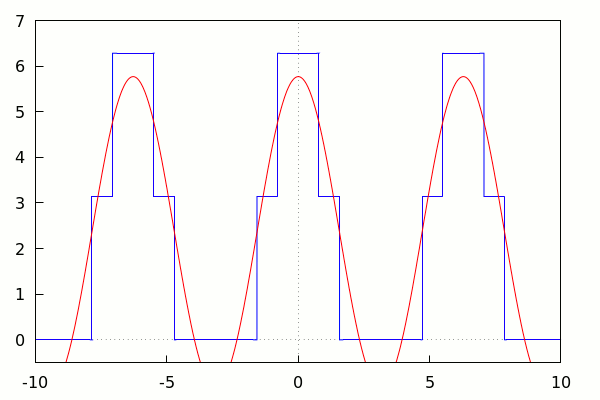
Définition de la fonction en fragments :

  • 2Pi pour 0 <= t < Pi/4
  • Pi pour Pi/4 <= t < Pi/2
  • 0 pour Pi/2 <= t < Pi


–>

f(t) :=

if t>=0 and t < %pi/4 then 2·%pi

else if t>=%pi/4 and t < %pi/2 then %pi

else if t>=%pi/2 and t <= %pi then 0

else if t<0 and t>=%pi then f(t)

else if t>0 then f(t ceiling(t/(2·%pi))·2·%pi)

else if t<0 then f(t);

\[\tag{%o35} \operatorname{f}(t):=\operatorname{if} t\mbox{> =}0\mathit{ and }t\mbox{< }\frac{\ensuremath{\pi} }{4} \operatorname{then} 2 \ensuremath{\pi} \operatorname{else} \operatorname{if} t\mbox{> =}\frac{\ensuremath{\pi} }{4}\mathit{ and }t\mbox{< }\frac{\ensuremath{\pi} }{2} \operatorname{then} \ensuremath{\pi} \operatorname{else} \operatorname{if} t\mbox{> =}\frac{\ensuremath{\pi} }{2}\mathit{ and }t\mbox{< =}\ensuremath{\pi} \operatorname{then} 0 \operatorname{else} \operatorname{if} t\mbox{< }0\mathit{ and }t\mbox{> =}-\ensuremath{\pi} \operatorname{then} \operatorname{f}\left( -t\right) \operatorname{else} \operatorname{if} t\mbox{> }0 \operatorname{then} \operatorname{f}\left( t-\operatorname{ceiling}\left( \frac{t}{2 \ensuremath{\pi} }\right) 2 \ensuremath{\pi} \right) \operatorname{else} \operatorname{if} t\mbox{< }0 \operatorname{then} \operatorname{f}\left( -t\right) \]


–>

f(4.9);

\[\tag{%o2} \ensuremath{\pi} \]


Courbe ( 3 périodes )


–>

wxplot2d( f(t), [t, 10, 10], [xtics, %pi], [title, "signal"]);

\[\tag{%t36} \]
 (Graphics)

\[\tag{%o36} \]


–>

load("draw");

\[\mbox{}\\\mbox{0 errors, 0 warnings}\]
\[\tag{%o38} /usr/local/share/maxima/5.41.0/share/draw/draw.lisp\]


Définition d’une fonction fsignal, paramétrée par n = nombre de termes de la série de fourier à prendre en considération


–>

fsignal(n, x)  := block([i],

res : 3·%pi/4,

for i from 1 thru n do (

     res : res + (2/i) · ( sin(i·%pi/4) + sin(i·%pi/2)) · cos(i·x)

),

res);

\[\tag{%o39} \operatorname{fsignal}\left( n,x\right) :=\operatorname{block}\left( [i],\mathit{res}:\frac{3 \ensuremath{\pi} }{4},\operatorname{for} i \operatorname{thru} n \operatorname{do} \mathit{res}:\mathit{res}+\frac{2}{i}\, \left( \sin{\left( \frac{i \ensuremath{\pi} }{4}\right) }+\sin{\left( \frac{i \ensuremath{\pi} }{2}\right) }\right) \cos{\left( i x\right) },\mathit{res}\right) \]


–>

fsignal(1,x);

\[\tag{%o40} 2 \left( \frac{1}{\sqrt{2}}+1\right) \cos{(x)}+\frac{3 \ensuremath{\pi} }{4}\]


–>

set_draw_defaults(

  xaxis = true, xaxis_color = red,

  xaxis_type = solid, xaxis_width = 1,  xtics=1,

  yaxis = true, yaxis_color = red, ytics=1,

  yaxis_type = solid, yaxis_width = 1,

  dimensions = [600,600],

  grid = true,

  nticks = 150,

  ip_grid = [100,100],

  line_width = 3

);


\[\tag{%o41} [\mathit{xaxis}=\mbox{true},\mathit{xaxis\_ color}=\mathit{red},\mathit{xaxis\_ type}=\mathit{solid},\mathit{xaxis\_ width}=1,\mathit{xtics}=1,\mathit{yaxis}=\mbox{true},\mathit{yaxis\_ color}=\mathit{red},\mathit{ytics}=1,\mathit{yaxis\_ type}=\mathit{solid},\mathit{yaxis\_ width}=1,\mathit{dimensions}=[600,600],\mathit{grid}=\mbox{true},\mathit{nticks}=150,\mathit{ip\_ grid}=[100,100],\mathit{line\_ width}=3]\]


Traçage de la fonction ‘signal’ et de la somme Fourier au rang  n = 20


–>

wxdraw2d(color=blue,line_width=2,

    explicit(fsignal(20,x),x,10,10),

    color=red,

    explicit(f(x), x, 10, 10)

   );

\[\tag{%t42} \]
 (Graphics)

\[\tag{%o42} \]


–>

with_slider_draw(k, makelist(i, i, 1, 15),

   xrange=[10, 10], yrange=[0.5, 7],

   xaxis = true, yaxis = true,

   color = blue, explicit(f(x), x, 10, 10),

   color = red, explicit(fsignal(k,x),x,10,10)

);

\[\tag{%t11} \]
Animated Diagram
\[\tag{%o11} \]


–>

makelist(1/n·cos(n·%pi/4) +1/n·cos(n·%pi/2), n, 1, 6);

\[\tag{%o13} [\frac{1}{\sqrt{2}},-\frac{1}{2},-\frac{1}{3 \sqrt{2}},0,-\frac{1}{5 \sqrt{2}},-\frac{1}{6}]\]